|
|
5.准备工作(二)
5.1.错误纠正
在上文中,我介绍了数据框架的搭建思路,给出了一部分的Barra风格因子计算的代码。但是,在写博客时,存在一些表述不完善的地方。在此我做一下更正:
- “至今为止,无人在网络上发布因子计算代码”表述有误,我在Github上找到了别人发布的因子计算代码:
- 在写上篇博客时,我没找到MSCI原文,但后来在人大经济论坛中找到了一个含有原文的压缩包:
5.2.数据补充
在后面风格因子的计算过程中,我发现原有底层数据不足以支撑后续的因子计算。一是聚宽单季度财务数据字段不全面,二是还缺乏分析师的一致预期数据。
5.2.1.分析师数据
首先解决分析师一致预期数据。有许多平台提供了分析师的一致预期,如Wind、朝阳永续、tushare、CSMAR等等。在考虑使用哪个数据源时,主要需要考虑以下几个方面。一是数据源质量,如果数据的时间范围有限、数据搜集不全面,则要考虑更换数据源;二是数据获取权限,即每天能够获取的数据量能覆盖当天的新增数据;三是数据更新频率,因子数据需要实时更新,辅助投资决策,如果数据更新频率太低,则不适合。四是要考虑是否具有数据接口,如果数据平台没有提供数据接口,只提供数据文件的下载,那么只能手动更新,比较麻烦。
综合考虑,我选用tushare作为我的分析师一致预期数据库的数据源,数据提取说明见tushare数据接口文档:
自己本地的数据提取函数为get_report,参数说明如下:
def get_report(codes=None, start_date=None, end_date=None, count=365, year=None, fields=None):
"""
获取股票研究报告数据。
codes:list,股票代码列表;
start_date/end_date:datetime or str,研究报告发布的开始日期、结束日期;
count:自然日个数,当start_date/end_date不完全指定的时候使用
year:int or str or list[str|int],指定提取预期年份,如2023年预期数据。
fields:list,需要提取的字段列表,默认全取。可以通过get_field_description获取字段说明。
"""
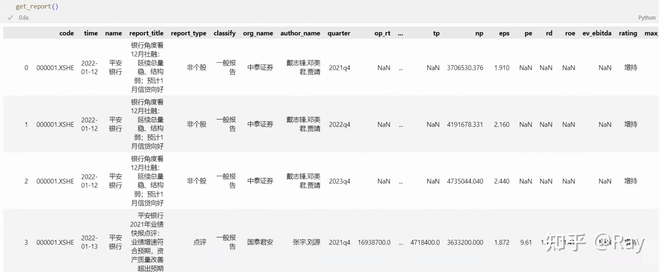
get_report函数运行结果
上图展示的是get_report函数的运行结果。code、time分别是股票代码和研究报告的发布时间。后续的字段比较好理解,这里不再赘述。
一份研究报告一般预测还未发布的三年的财务数据。以中泰证券2022-01-12发布的研究报告为例(图中0、1、2行),其预测了2021q4、2022q4和2023q4。而2021q4在那时已经过去,但2021q4的财务报表还未发布,所以证券研究报告依然对其进行了预测。
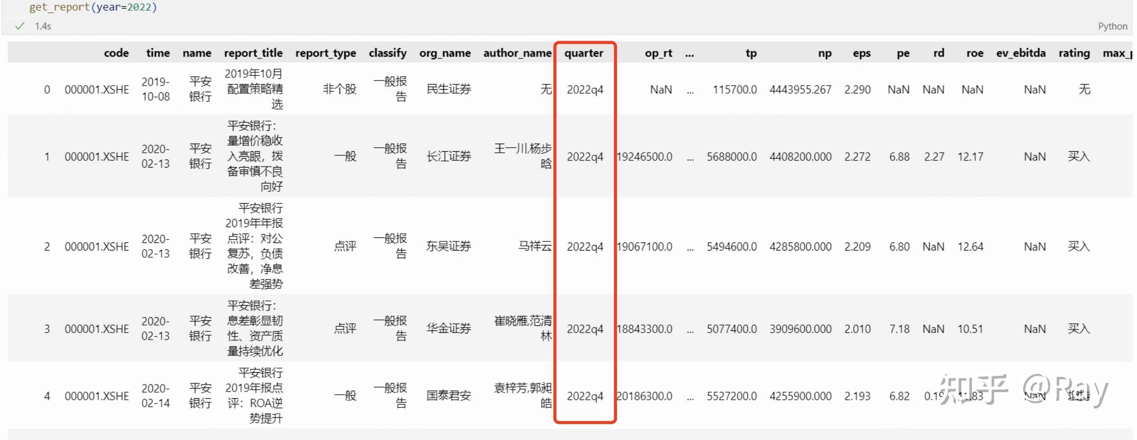
如下图,如果我只需要关于2022q4的财务数据预测,我只需要指定参数year=2022即可。
指定年份获取研究报告数据
5.2.2.三大报表完整数据
然后,解决季度财务报表字段不全的问题。聚宽存在两套财务数据,一套是按季度计算的财务数据,即前文中提到的四张基本面数据表格;另一套是完整的三大报表数据,数据字段说明见聚宽文档:
https://www.joinquant.com/help/api/help#Stock:合并利润表
https://www.joinquant.com/help/api/help#Stock:合并现金流量表
https://www.joinquant.com/help/api/help#Stock:合并资产负债表
对于上述数据,我分别做了数据提取与接口开发,分别编写了三个本地数据接口函数get_income、get_cashflow和get_balance。并将数据源整合到上一篇文章的get_basic函数。代码参数展示如下:
def get_balance(codes=None, start_date=None, end_date=None, count=4, fields=None, is_full=False):
"""
获取资产负债表相关数据。
codes: 股票代码,list,默认获取全部。
start_date/end_date: 开始和结束日期,默认为空。
count: 默认为4,代表取最近4个季度的数据。
fields: 相关字段,默认全取。可以使用`get_field_descrition`获取字段说明。
is_full: 是否提取完整的财务报表
"""
def get_cashflow(codes=None, start_date=None, end_date=None, count=4, fields=None, is_full=False):
"""
获取现金流量表相关数据。
codes: 股票代码,list,默认获取全部。
start_date/end_date: 开始和结束日期,默认为空。
count: 默认为4,代表取最近4个季度的数据。
fields: 相关字段,默认全取。可以使用`get_field_descrition`获取字段说明。
is_full: 是否提取完整的财务报表
"""
def get_income(codes=None, start_date=None, end_date=None, count=4, fields=None, is_full=False):
"""
获取利润表相关数据。
codes: 股票代码,list,默认获取全部。
start_date/end_date: 开始和结束日期,默认为空。
count: 默认为4,代表取最近4个季度的数据。
fields: 相关字段,默认全取。可以使用`get_field_descrition`获取字段说明。
is_full: 是否提取完整的财务报表
"""
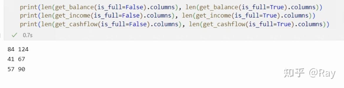
从运行结果来看,完整报表的字段更加全面。
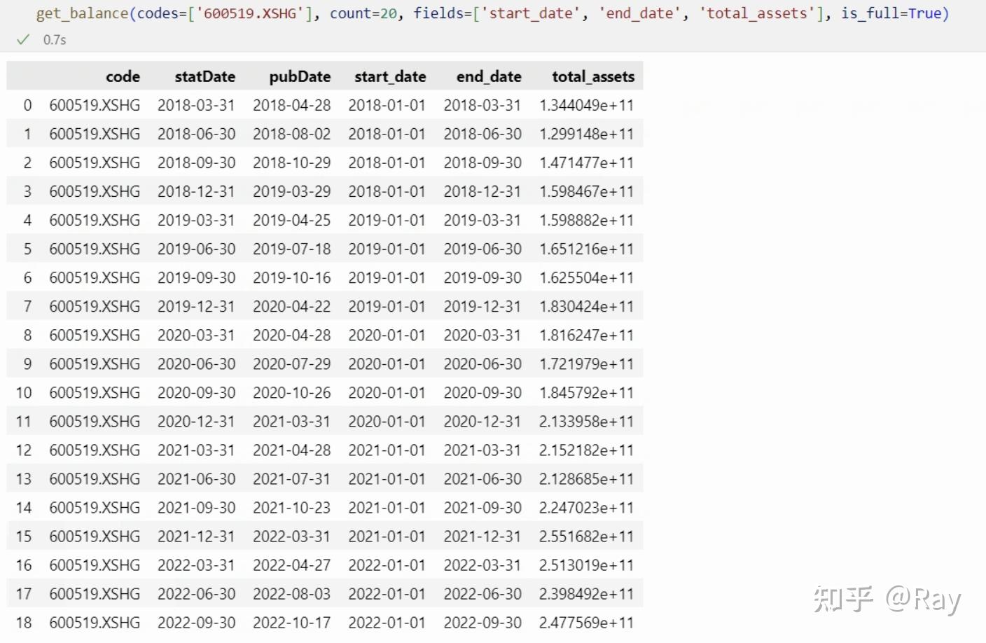
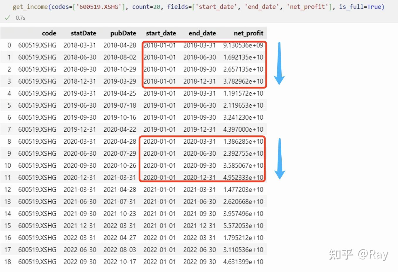
接下来描述数据结构。众所周知,资产负债表描述的是存量数据,即报告期末公司的资产负债情况;而现金流量表、利润表均为流量数据,有时间段的概念。所以资产负债表的字段数据只随结束时间(报告期)的不同而变化,而现金流量表、利润表字段数据受到开始时间、结束时间的影响。
我们以贵州茅台(代码600519.XSHG)的数据为例,尝试提取数据。其中code、statDate、pubDate分别为股票代码、报告期、发布日期,为固定字段,而start_date、end_date为财务报告的开始时间和结束时间。
资产负债表字段数据样本
可见,对于资产负债表的字段,其不受开始时间的影响,是一个截面数据、存量数据。
然后,我们来看看贵州茅台的净利润数据。可以发现流量数据都是按年度、以累计形式记录。
净利润数据为按年累计形式
再看看比较“冷门”的字段。我们来提取计算折旧摊销需要的字段。折旧摊销=固定资产折旧、油气资产折耗、生产性生物资产折旧+无形资产摊销+长期待摊费用摊销。
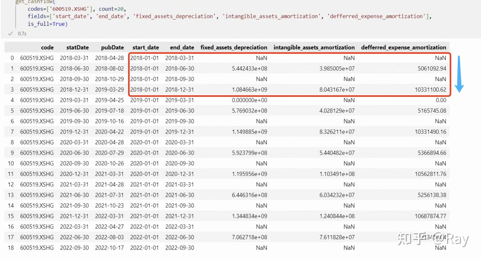
折旧摊销的计算字段
发现了什么?折旧摊销的计算字段每半年才公布一次数据,以累计形式公布。也即我们在计算折旧摊销相关的因子数据时,必须将数据频率降低,将季度频率降低到半年度频率。这时候插值、减半都是不合适的,因为这会引入未来数据。
5.3.小寄巧补充
5.3.1.带半衰期的权重计算
在上一篇文章中讲述了这个权重的计算方法。在后续的因子计算过程中,发现需要频繁地求这个权重,所以将这个权重的计算方法整合成一个函数。
import numpy as np
def get_exponent_weight(window, half_life, is_standardize=True):
L, Lambda = 0.5**(1/half_life), 0.5**(1/half_life)
W = []
for i in range(window):
W.append(Lambda)
Lambda *= L
W = np.array(W[::-1])
if is_standardize:
W /= np.sum(W)
return W
5.3.2.公布日对齐交易日
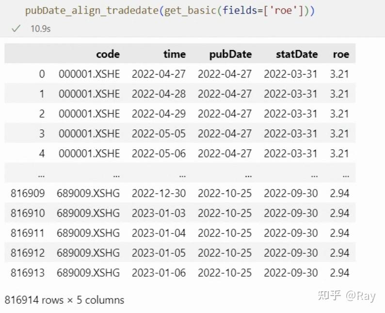
无论是财务报表还是研究报告,都有一个发布日期,在发布日期之后我们才知晓公司的这个数据。所以,为了将数据对齐,我设计了一个函数。(global_end_date是全局的截止日期,保存在我的数据库中)
def pubDate_align_tradedate(df, pubDate_col='pubDate', end_date=global_end_date):
"""将DataFrame中的公告时间与交易时间对应"""
def __custom_ffill(x):
x['time.1'] = x['time'].copy()
idx = x['time'].isna()
x.loc[idx, 'time'] = x.loc[idx, pubDate_col]
return x.sort_values(by='time').ffill().dropna().drop(columns='time.1')
trade_date = get_trade_date(start_date=df[pubDate_col].min(), end_date=end_date)
time_code = []
for i in trade_date:
for j in df['code'].unique():
time_code.append([i, j])
trade_date = pd.DataFrame(time_code, columns=['time', 'code'])
trade_date['time'] = pd.to_datetime(trade_date['time'])
res = df.merge(trade_date, left_on=['code', 'pubDate'], right_on=['code', 'time'], how='outer')
res = res.groupby('code', as_index=False).apply(__custom_ffill).reset_index(drop=True)
fix_field = ['code', 'time', pubDate_col]
fields = fix_field + [c for c in res.columns if c not in fix_field]
return res[fields]
假如将公司的季度ROE用作股票的业绩因子暴露,需要将ROE的发布时间对齐交易日,可以这样操作:
5.3.3.面板数据的rolling.apply
面板数据包含个体列、时间列以及数值列。如果我们需要在时间维度,对所有个体的数据计算移动窗口,再返回面板格式的数据,则可以使用这个函数。
此函数的操作步骤分成三步:
- 收到数据后先转化矩阵数据,以时间列为index,个体列为columns。
- 对矩阵数据进行移动窗口(rolling),然后施加某种操作(apply)。
- 操作完成后还原成面板数据,并去除缺失值。
import pandas as pd
import numpy as np
from functools import wraps
from joblib import Parallel, delayed
def try_except(func):
@wraps(func)
def decorated(*args, **kargs):
try:
return func(*args, **kargs)
except:
return np.nan
return decorated
def panel_rolling_apply(
df, time_col, id_col, value_col, window, apply_func, rolling_kargs={},
dropna=True, fillna_value=None, fillna_method='ffill', parallel=False, min_periods=None
):
"""面板数据转换成矩阵数据,rolling apply,然后再转换回面板数据。支持并行。"""
if min_periods is None:
min_periods = window
@try_except
def __apply_func(group):
group_name = group.index[-1]
if len(group)<min_periods:
return pd.Series(np.nan, index=group.columns, name=group_name)
group = apply_func(group, axis=0)
group.name = group_name
return group
tmp = pd.pivot_table(df, values=value_col, index=time_col, columns=id_col)
tmp_rolling = tmp.rolling(window, **rolling_kargs)
if parallel:
tmp = Parallel(12)(delayed(__apply_func)(group) for group in tmp_rolling)
tmp = pd.concat(tmp, axis=1).T
tmp.index.name = time_col
else:
tmp = tmp_rolling.apply(apply_func)
if (fillna_value is not None) ^ (fillna_method is not None):# 逻辑异或
tmp = tmp.fillna(fillna_value, method=fillna_method)
if dropna:
tmp = tmp.dropna(how=&#39;all&#39;)
return pd.melt(tmp.reset_index(), id_vars=time_col, value_name=value_col)\
.dropna().reset_index(drop=True)
6.动量(Momentum)
6.1.因子定义
此环节仅展示因子分级的结构,详细定义见代码实现。
- Momentum(一级因子)
- Short Term reversal(二级因子)
- Short Term reversal(三级因子):短期反转。最近一个月的加权累积对数日收益率。
- Seasonality(二级因子)
- Seasonality(三级因子):季节因子。过去五年的已实现次月收益率的平均值。
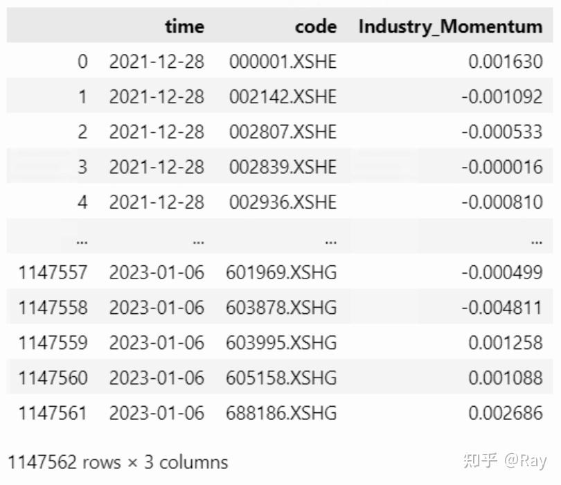
- Industry Momentum(二级因子)
- Industry Momentum(三级因子):行业动量。该指标描述个股相对中信一级行业的强度。(但我的数据库中没有中信一级行业,所以改用申万一级行业)
- Momentum(二级因子)
- Relative strength(三级因子):相对于市场的强度。
- Historical alpha(三级因子):在BETA计算所进行的时间序列回归中取回归截距项。(那改一改前面的代码,这里就不算了)
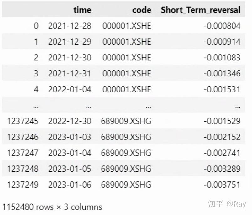
6.2.Short Term reversal
短期反转的公式定义如下:
STREV(t)=\sum_{\tau \in T} w_{\tau-t-1}[\ln(1+r(\tau))] \\
其中,r为过去21天的股票收益率的算术平均数;w为半衰指数权重,时间窗口为21个交易日,半衰期为5个交易日;T=\{t-1, \dots, t-n\}
首先,我们使用如下代码获取股票收益率数据,经过简单处理,收益率数据呈矩阵形式:
codes=None
start_date=None
end_date=None
count=250
s, end_date = __start_end_date__(start_date=start_date, end_date=end_date, count=count)
if codes is None:
codes_ = &#39;all-stock&#39;
# 短期反转
s1, _ = __start_end_date__(start_date=None, end_date=s, count=41)
price1 = get_price(codes=codes_, start_date=s1, end_date=end_date, fields=[&#39;close&#39;, &#39;pre_close&#39;])
price1[&#39;ret&#39;] = price1[&#39;close&#39;] / price1[&#39;pre_close&#39;] - 1
ret = pd.pivot_table(price1, values=&#39;ret&#39;, index=&#39;time&#39;, columns=&#39;code&#39;)
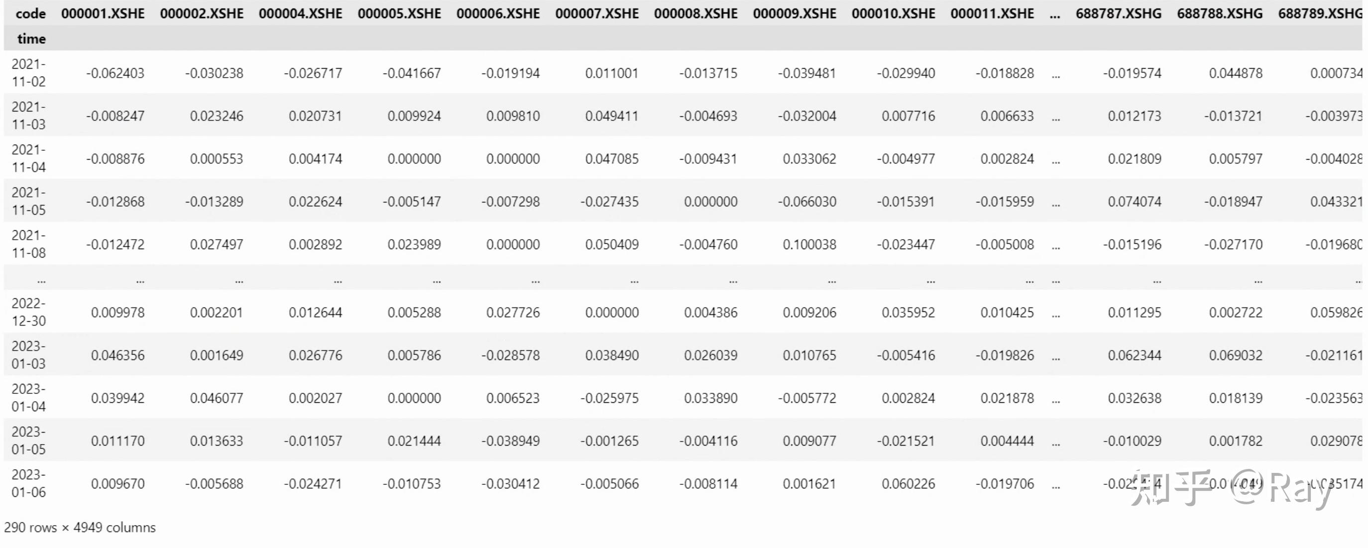
收益率矩阵
然后,计算因子:
r_n = ret.rolling(21).mean().dropna(how=&#39;all&#39;)
W = get_exponent_weight(window=21, half_life=5)
STREV = []
for i in range(len(r_n)-20):
tmp = np.log(1 + r_n.iloc[i:i+21, :].copy())
tmp = pd.Series(np.sum(W.reshape(-1, 1)*tmp.values, axis=0), name=tmp.index[-1], index=tmp.columns)
STREV.append(tmp)
STREV = pd.concat(STREV, axis=1).T
STREV.index.name = &#39;time&#39;
STREV = pd.melt(STREV.reset_index(), id_vars=&#39;time&#39;, value_name=&#39;Short_Term_reversal&#39;).dropna()
6.3.Seasonality
季节因子被定义为过去五年的已实现次月收益率的平均值。我们直接获取后复权收盘价即可实现计算:
# 季节因子
trade_date = get_trade_date(start_date=s, end_date=end_date)
season = {}
for td in track(trade_date, description=&#39;正在计算季节性⋯⋯&#39;):
r_y = []
for i in range(1, 6):
td_shift = get_trade_date(start_date=td-pd.Timedelta(days=365*i), count=21)
s_, e_ = td_shift[0], td_shift[-1]
p_ = get_price(codes=codes_, start_date=s_, end_date=e_, fields=[&#39;close&#39;])
p_ = pd.pivot_table(p_, index=&#39;time&#39;, columns=&#39;code&#39;, values=&#39;close&#39;).ffill()
r_y.append(p_.iloc[-1, :] / p_.iloc[0, :] - 1)
season[pd.to_datetime(td)] = pd.concat(r_y, axis=1).mean(axis=1)
season = pd.DataFrame(season).T
season.index.name = &#39;time&#39;
season = pd.melt(season.reset_index(), id_vars=&#39;time&#39;, value_name=&#39;Seasonality&#39;)
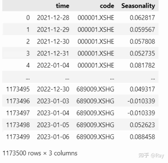
为了保证因子覆盖度,基本上,上市一年以上的股票就有因子数值。这个设定可能是不合理的,后续再改改。
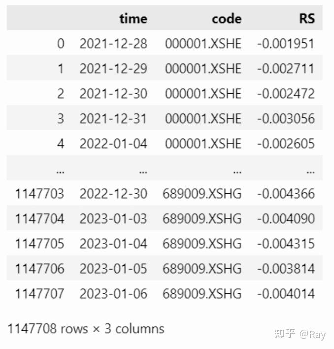
6.4.Industry Momentum
该因子的计算过程分为三步。
首先给出了个股相对强度的定义:
RS_S(t)=\sum_{\tau \in T(t)}w_{\tau-t}[\ln(1+r_S(\tau))] \\
其中,r_S为日度股票收益率,w为半衰指数权重,时间窗口为6个月,半衰期为1个月,T=\{t, \dots ,t-n\}ra
然后,给出行业I_t的相对强度定义:
RS_I(t)=\sum_{i\in I(t)}c_i(t)RS_i(t) \\
其中,c_i(t)是个股i的流通市值平方根。
最后,行业动量定义为:
\mathrm{INDMOM}_S(t)=-(c_S(t)RS_S(t)-RS_I(t)) \\
我认为这个指标容易受到行业市值的影响,在截面上不同行业之间可能没有选股能力,所以我将权重c_i(t)做了如下修改:
c_i(t):=\frac{c_i(t)}{\sum_{i \in I(t)} c_i(t)} \\
代码实现如下,首先计算个股强度:
# 行业动量
s2, _ = __start_end_date__(start_date=None, end_date=s, count=126)
price = get_price(codes=codes_, start_date=s2, end_date=end_date, fields=[&#39;pre_close&#39;, &#39;close&#39;])
price[&#39;ret&#39;] = price[&#39;close&#39;] / price[&#39;pre_close&#39;] - 1
ret = pd.pivot_table(price, index=&#39;time&#39;, columns=&#39;code&#39;, values=&#39;ret&#39;)
W = get_exponent_weight(window=126, half_life=21)
RS = {}
for i in track(range(len(ret)-125), description=&#39;正在计算个股强度⋯⋯&#39;):
tmp = ret.iloc[i:i+126, :].copy()
# 缺失值在10%以内
tmp = tmp.loc[:, tmp.isnull().sum(axis=0) / 252 <= 0.1].fillna(0.)
tmp = np.log(1 + tmp)
RS[tmp.index[-1]] = pd.Series(np.sum(W.reshape(-1, 1)*tmp.values, axis=0), index=tmp.columns)
RS = pd.DataFrame(RS).T
RS.index.name = &#39;time&#39;
RS = pd.melt(RS.reset_index(), id_vars=&#39;time&#39;, value_name=&#39;RS&#39;).dropna().reset_index(drop=True)
然后计算行业相对强度,并计算指标:
def __industry_RS(x):
ind_RS = x.groupby(&#39;industry_name&#39;).apply(
lambda y: y[&#39;RS&#39;].dot(y[&#39;c&#39;]) / y[&#39;c&#39;].sum()
)
ind_RS.name = &#39;ind_RS&#39;
ind_RS = ind_RS.reset_index()
x = pd.merge(x, ind_RS)
x[&#39;Industry_Momentum&#39;] = x[&#39;ind_RS&#39;] - x[&#39;RS&#39;]
return x[[&#39;code&#39;, &#39;Industry_Momentum&#39;]].set_index(&#39;code&#39;)
val = get_valuation(start_date=s, end_date=end_date, fields=[&#39;circulating_market_cap&#39;])
RS = pd.merge(RS, val)
RS[&#39;mon&#39;] = RS[&#39;time&#39;].apply(lambda x: x.strftime(&#34;%Y-%m-01&#34;))
RS[&#39;c&#39;] = np.sqrt(RS[&#39;circulating_market_cap&#39;])
INDMOM = []
for m, tmp_RS in track(RS.groupby(&#39;mon&#39;), description=&#39;正在计算行业动量⋯⋯&#39;):
ind = get_industry(date=m, industry_type=[&#39;sw_l1&#39;])[[&#39;code&#39;, &#39;industry_name&#39;]]
tmp_RS = pd.merge(tmp_RS, ind)
INDMOM.append(tmp_RS.groupby(&#39;time&#39;).apply(__industry_RS).reset_index())
INDMOM = pd.concat(INDMOM).reset_index(drop=True)
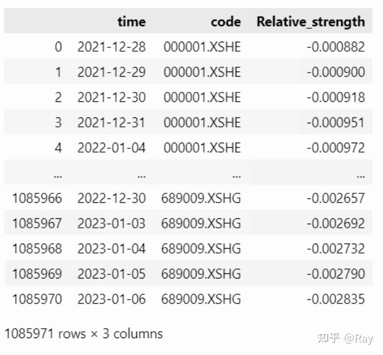
6.5.Relative strength
计算非滞后的相对强度:对股票的对数收益率进行半衰指数加权求和,时间窗口252个交易日,半衰期126个交易日。然后,以11个交易日为窗口,滞后11个交易日,取非滞后相对强度的等权平均值。
代码实现如下:
# 相对强度
s3, _ = __start_end_date__(start_date=None, end_date=s, count=262)
W = get_exponent_weight(window=252, half_life=126)
price = get_price(codes=codes_, start_date=s3, end_date=end_date, fields=[&#39;pre_close&#39;, &#39;close&#39;])
price[&#39;ret&#39;] = np.log(price[&#39;close&#39;]) - np.log(price[&#39;pre_close&#39;])
ret = pd.pivot_table(price, index=&#39;time&#39;, columns=&#39;code&#39;, values=&#39;ret&#39;)
Relative_strength = {}
for i in track(range(len(ret) - 251), description=&#39;正在计算非滞后相对强度⋯⋯&#39;):
tmp = ret.iloc[i:i+252, :]
tmp = tmp.loc[:, tmp.isnull().sum(axis=0) / 252 <= 0.1].fillna(0.)
np.sum(W.reshape(-1, 1)*tmp.values, axis=0)
Relative_strength[tmp.index[-1]] = pd.Series(np.sum(W.reshape(-1, 1)*tmp.values, axis=0), index=tmp.columns)
Relative_strength = pd.DataFrame(Relative_strength).T
Relative_strength.index.name = &#39;time&#39;
Relative_strength = Relative_strength.rolling(11).mean().dropna(how=&#39;all&#39;)
Relative_strength = pd.melt(Relative_strength.reset_index(), id_vars=&#39;time&#39;, value_name=&#39;Relative_strength&#39;).dropna().reset_index(drop=True)
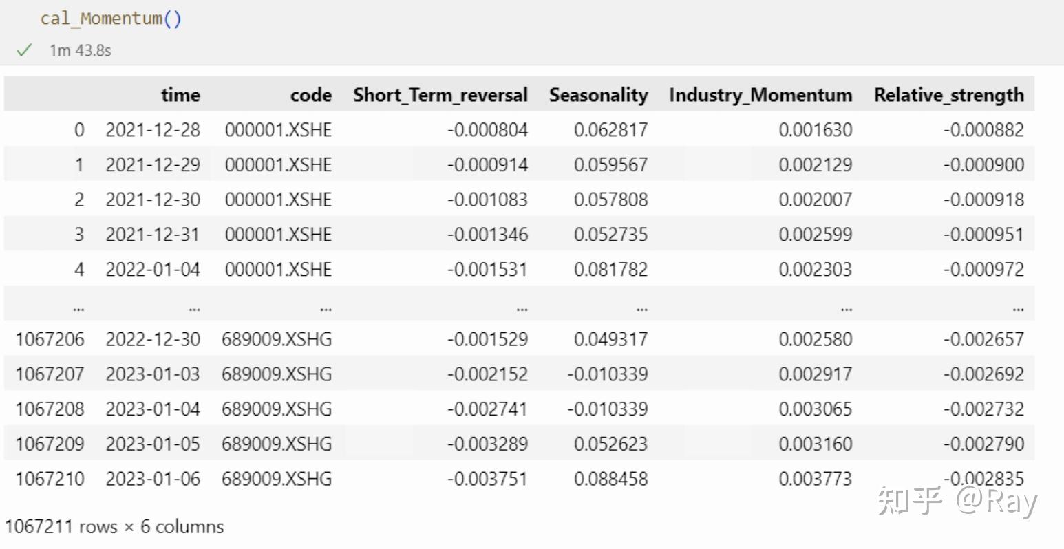
6.6.代码整合
我们将上述代码整理成一个函数:
from rich.progress import track
import pandas as pd
from IPython.display import clear_output
def cal_Momentum(codes=None, start_date=None, end_date=None, count=250):
s, end_date = __start_end_date__(start_date=start_date, end_date=end_date, count=count)
if codes is None:
codes_ = &#39;all-stock&#39;
# 短期反转
s1, _ = __start_end_date__(start_date=None, end_date=s, count=41)
price1 = get_price(codes=codes_, start_date=s1, end_date=end_date, fields=[&#39;close&#39;, &#39;pre_close&#39;])
price1[&#39;ret&#39;] = price1[&#39;close&#39;] / price1[&#39;pre_close&#39;] - 1
ret = pd.pivot_table(price1, values=&#39;ret&#39;, index=&#39;time&#39;, columns=&#39;code&#39;)
r_n = ret.rolling(21).mean().dropna(how=&#39;all&#39;)
W = get_exponent_weight(window=21, half_life=5)
STREV = []
for i in range(len(r_n)-20):
tmp = np.log(1 + r_n.iloc[i:i+21, :].copy())
tmp = pd.Series(np.sum(W.reshape(-1, 1)*tmp.values, axis=0), name=tmp.index[-1], index=tmp.columns)
STREV.append(tmp)
STREV = pd.concat(STREV, axis=1).T
STREV.index.name = &#39;time&#39;
STREV = pd.melt(STREV.reset_index(), id_vars=&#39;time&#39;, value_name=&#39;Short_Term_reversal&#39;).dropna()
# 季节因子
trade_date = get_trade_date(start_date=s, end_date=end_date)
season = {}
for td in track(trade_date, description=&#39;正在计算季节性⋯⋯&#39;):
r_y = []
for i in range(1, 6):
td_shift = get_trade_date(start_date=td-pd.Timedelta(days=365*i), count=21)
s_, e_ = td_shift[0], td_shift[-1]
p_ = get_price(codes=codes_, start_date=s_, end_date=e_, fields=[&#39;close&#39;])
p_ = pd.pivot_table(p_, index=&#39;time&#39;, columns=&#39;code&#39;, values=&#39;close&#39;).ffill()
r_y.append(p_.iloc[-1, :] / p_.iloc[0, :] - 1)
season[pd.to_datetime(td)] = pd.concat(r_y, axis=1).mean(axis=1)
season = pd.DataFrame(season).T
season.index.name = &#39;time&#39;
season = pd.melt(season.reset_index(), id_vars=&#39;time&#39;, value_name=&#39;Seasonality&#39;)
factor = pd.merge(STREV, season)
# 行业动量
s2, _ = __start_end_date__(start_date=None, end_date=s, count=126)
price = get_price(codes=codes_, start_date=s2, end_date=end_date, fields=[&#39;pre_close&#39;, &#39;close&#39;])
price[&#39;ret&#39;] = price[&#39;close&#39;] / price[&#39;pre_close&#39;] - 1
ret = pd.pivot_table(price, index=&#39;time&#39;, columns=&#39;code&#39;, values=&#39;ret&#39;)
W = get_exponent_weight(window=126, half_life=21)
RS = {}
for i in track(range(len(ret)-125), description=&#39;正在计算个股强度⋯⋯&#39;):
tmp = ret.iloc[i:i+126, :].copy()
# 缺失值在10%以内
tmp = tmp.loc[:, tmp.isnull().sum(axis=0) / 252 <= 0.1].fillna(0.)
tmp = np.log(1 + tmp)
RS[tmp.index[-1]] = pd.Series(np.sum(W.reshape(-1, 1)*tmp.values, axis=0), index=tmp.columns)
RS = pd.DataFrame(RS).T
RS.index.name = &#39;time&#39;
RS = pd.melt(RS.reset_index(), id_vars=&#39;time&#39;, value_name=&#39;RS&#39;).dropna().reset_index(drop=True)
val = get_valuation(start_date=s, end_date=end_date, fields=[&#39;circulating_market_cap&#39;])
RS = pd.merge(RS, val)
RS[&#39;mon&#39;] = RS[&#39;time&#39;].apply(lambda x: x.strftime(&#34;%Y-%m-01&#34;))
RS[&#39;c&#39;] = np.sqrt(RS[&#39;circulating_market_cap&#39;])
def __industry_RS(x):
ind_RS = x.groupby(&#39;industry_name&#39;).apply(
lambda y: y[&#39;RS&#39;].dot(y[&#39;c&#39;]) / y[&#39;c&#39;].sum()
)
ind_RS.name = &#39;ind_RS&#39;
ind_RS = ind_RS.reset_index()
x = pd.merge(x, ind_RS)
x[&#39;Industry_Momentum&#39;] = x[&#39;ind_RS&#39;] - x[&#39;RS&#39;]
return x[[&#39;code&#39;, &#39;Industry_Momentum&#39;]].set_index(&#39;code&#39;)
INDMOM = []
for m, tmp_RS in track(RS.groupby(&#39;mon&#39;), description=&#39;正在计算行业动量⋯⋯&#39;):
ind = get_industry(date=m, industry_type=[&#39;sw_l1&#39;])[[&#39;code&#39;, &#39;industry_name&#39;]]
tmp_RS = pd.merge(tmp_RS, ind)
INDMOM.append(tmp_RS.groupby(&#39;time&#39;).apply(__industry_RS).reset_index())
INDMOM = pd.concat(INDMOM).reset_index(drop=True)
factor = factor.merge(INDMOM)
# 相对强度
s3, _ = __start_end_date__(start_date=None, end_date=s, count=262)
W = get_exponent_weight(window=252, half_life=126)
price = get_price(codes=codes_, start_date=s3, end_date=end_date, fields=[&#39;pre_close&#39;, &#39;close&#39;])
price[&#39;ret&#39;] = np.log(price[&#39;close&#39;]) - np.log(price[&#39;pre_close&#39;])
ret = pd.pivot_table(price, index=&#39;time&#39;, columns=&#39;code&#39;, values=&#39;ret&#39;)
Relative_strength = {}
for i in track(range(len(ret) - 251), description=&#39;正在计算非滞后相对强度⋯⋯&#39;):
tmp = ret.iloc[i:i+252, :]
tmp = tmp.loc[:, tmp.isnull().sum(axis=0) / 252 <= 0.1].fillna(0.)
np.sum(W.reshape(-1, 1)*tmp.values, axis=0)
Relative_strength[tmp.index[-1]] = pd.Series(np.sum(W.reshape(-1, 1)*tmp.values, axis=0), index=tmp.columns)
Relative_strength = pd.DataFrame(Relative_strength).T
Relative_strength.index.name = &#39;time&#39;
Relative_strength = Relative_strength.rolling(11).mean().dropna(how=&#39;all&#39;)
Relative_strength = pd.melt(Relative_strength.reset_index(), id_vars=&#39;time&#39;, value_name=&#39;Relative_strength&#39;).dropna().reset_index(drop=True)
factor = factor.merge(Relative_strength)
clear_output()
return factor
cal_Momentum()
7.质量(Quality)(一)
此因子工作量较大,剩余部分将放在下一篇文章展示,喜欢的话可以点个关注。
因子结构如下:
- Quality(一级因子)
- Leverage(二级因子)
- Market Leverage(三级因子):市场杠杆
- Book Leverage(三级因子):账面杠杆
- Debt to asset ratio(三级因子):资产负债比
- Earning Variability(二级因子)
- Variation in Sales(三级因子):营业收入波动率
- Variation in Earning(三级因子):盈利波动率
- Variation in Cashflows(三级因子):现金流波动率
- Standard deviation of Analyst Forecast Earnings-to-Price(三级因子):分析师预测盈市率标准差
- Earnings Quality(二级因子)
- Accruals Balancesheet version(三级因子):资产负债表应计项目
- Accruals Cashflow version(三级因子):现金流量表应计项目
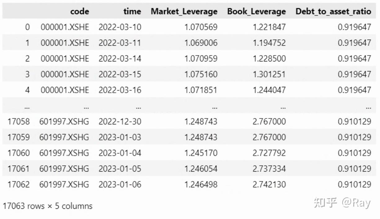
7.1.杠杆(Leverage)
二级因子杠杆下有三个三级因子,分别为市场杠杆、账面杠杆和资产负债比。其中,市场杠杆的计算公式为:
MLEV=\frac{ME+PE+LD}{ME} \\
账面杠杆的计算公式为:
BLEV=\frac{BE+PE+LD}{ME} \\
资产负债比的计算公式为:
DTOA=\frac{TL}{TA} \\
其中,ME为股票市值,BE为普通股账面价值,PE和LD分别是上一财政年度的优先股和长期负债,TL和TA分别为总负债和总资产。很显然,计算数据来源于资产负债表和valuation表格。
因子计算代码实现如下:
codes=None
start_date=None
end_date=None
count=250
s, end_date = __start_end_date__(start_date=start_date, end_date=end_date, count=count)
# 杠杆
s1, _ = __start_end_date__(start_date=None, end_date=s, count=270)
basic = get_basic(
codes=codes, start_date=s1, end_date=end_date,
fields=[
&#39;total_non_current_liability&#39;, # 长期负债
&#39;total_assets&#39;, &#39;total_liability&#39;, # 总资产、总负债
&#39;preferred_shares_equity&#39;, &#39;preferred_shares_noncurrent&#39; # 优先股
])
# 优先股单位调整
basic[&#39;PE&#39;] = (basic[&#39;preferred_shares_equity&#39;].fillna(0)+basic[&#39;preferred_shares_noncurrent&#39;].fillna(0))/1e8
# 长期负债单位调整
basic[&#39;LD&#39;] = (basic[&#39;total_non_current_liability&#39;] / 1e8).fillna(0)
# 交易日对齐
basic = pubDate_align_tradedate(basic.drop(columns=&#39;total_non_current_liability&#39;))
val = get_valuation(codes=codes, start_date=s, end_date=end_date, fields=[&#39;market_cap&#39;, &#39;pb_ratio&#39;])
factor = pd.merge(basic, val).rename(columns={&#39;market_cap&#39;: &#39;ME&#39;})
# pb值反推普通股账面价值
factor[&#39;BE&#39;] = factor[&#39;ME&#39;] / factor[&#39;pb_ratio&#39;]
# 因子计算
factor[&#39;Market_Leverage&#39;] = factor.eval(&#39;(ME+PE+LD)/ME&#39;)
factor[&#39;Book_Leverage&#39;] = factor.eval(&#39;(BE+PE+LD)/ME&#39;)
factor[&#39;Debt_to_asset_ratio&#39;] = factor.eval(&#39;total_liability/total_assets&#39;)
factor = factor[[&#39;code&#39;, &#39;time&#39;, &#39;Market_Leverage&#39;, &#39;Book_Leverage&#39;, &#39;Debt_to_asset_ratio&#39;]]
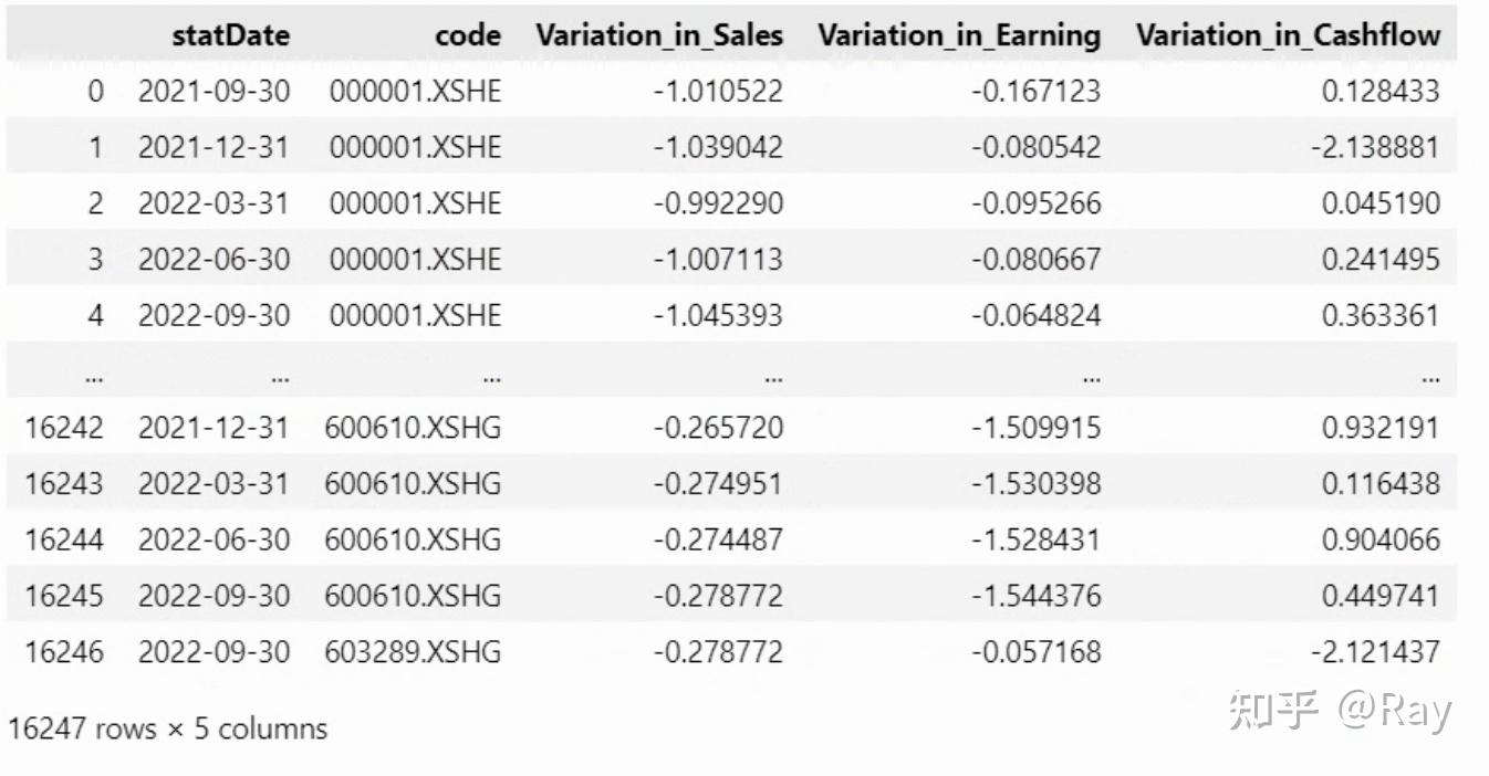
7.2.盈利波动(Earnings Variability)
因子的定义如下:
- Variation in Sales(三级因子):营业收入波动率。过去五个财年的年营业收入标准差除以平均年营业收入。
- Variation in Earning(三级因子):盈利波动率。过去五个财年的年净利润标准差除以平均年净利润。
- Variation in Cashflows(三级因子):现金流波动率。过去五个财年的年现金及现金等价物净增加额标准差除以平均年现金及现金等价物净增加额。
- Standard deviation of Analyst Forecast Earnings-to-Price(三级因子):分析师预测盈市率标准差。预测12月eps的标准差除以当前股价。
很显然,前三个因子来自利润表或现金流量表,可以一并计算。因为用于计算的字段不算“冷门”,可以计算季频因子。
先用代码实现前三个因子,并做5倍MAD调整、去均值方差处理:
import numpy as np
import pandas as pd
def MAD_winsorize(x, multiplier=5):
x_M = np.nanmedian(x)
x_MAD = np.nanmedian(np.abs(x-x_M))
upper = x_M + multiplier * x_MAD
lower = x_M - multiplier * x_MAD
x[x>upper] = upper
x[x<lower] = lower
return x
basic = get_basic(
start_date=pd.to_datetime(s)-pd.Timedelta(days=365*5+1), end_date=end_date,
fields=[&#39;operating_revenue&#39;, &#39;net_profit&#39;, &#39;cash_equivalent_increase&#39;])
def variation(x, **kargs):
return 4*np.nanstd(x) / np.nanmean(x)
def __modify(x):
vars_ = [&#39;Variation_in_Sales&#39;, &#39;Variation_in_Earning&#39;, &#39;Variation_in_Cashflow&#39;]
for v in vars_:
x[v] = MAD_winsorize(x[v].fillna(np.nanmedian(x[v])))
x[v] -= x[v].mean()
x[v] /= x[v].std()
return x
V_in_Sales = panel_rolling_apply(
basic, time_col=&#39;statDate&#39;, id_col=&#39;code&#39;, value_col=&#39;operating_revenue&#39;, window=20, apply_func=variation,
).rename(columns={&#39;operating_revenue&#39;: &#39;Variation_in_Sales&#39;})
V_in_Earning = panel_rolling_apply(
basic, time_col=&#39;statDate&#39;, id_col=&#39;code&#39;, value_col=&#39;net_profit&#39;, window=20, apply_func=variation
).rename(columns={&#39;net_profit&#39;: &#39;Variation_in_Earning&#39;})
V_in_Cashflow = panel_rolling_apply(
basic, time_col=&#39;statDate&#39;, id_col=&#39;code&#39;, value_col=&#39;cash_equivalent_increase&#39;, window=20, apply_func=variation
).rename(columns={&#39;cash_equivalent_increase&#39;: &#39;Variation_in_Cashflow&#39;})
factor_ = V_in_Sales.merge(V_in_Earning, how=&#39;outer&#39;).merge(V_in_Cashflow, how=&#39;outer&#39;)
# factor_ = pubDate_align_tradedate(factor_)[[&#39;code&#39;, &#39;time&#39;, &#39;Variation_in_Sales&#39;, &#39;Variation_in_Earning&#39;, &#39;Variation_in_Cashflow&#39;]]
factor_ = factor_.groupby(&#39;statDate&#39;).apply(__modify)
再来计算分析师EP波动率。该因子的计算方法为分析师预测当年12月eps的标准差除以当前股价。我认为这个数值可能不合理,因为股票分红、拆股等事件会影响股票股价,而分析师给出的eps预测只是基于当时的股票数量。所以,我将计算方法调整为分析师预测当年12月净利润的累计波动率,除以股票当天的市值。代码实现如下:
def __cumstd(x):
f_ = []
def __sub_cumstd(y, f_):
f_ += y[&#39;np&#39;].values.tolist()
if len(f_)<5:
return np.nan
return np.nanstd(f_)
np_std = x.groupby(&#39;time&#39;).apply(lambda z: __sub_cumstd(z, f_))
np_std.name = &#39;np_std&#39;
return np_std.dropna()
forecast_EP_std = []
for year in range(pd.to_datetime(s).year, pd.to_datetime(end_date).year+1):
forecast_np = get_report(end_date=f&#39;{year}-12-31&#39;, count=365*3, year=year, fields=[&#39;np&#39;])
forecast_np[&#39;np&#39;] /= 10000
np_std = forecast_np.groupby(&#39;code&#39;).apply(__cumstd).reset_index().rename(columns={&#39;time&#39;: &#39;pubDate&#39;})
np_std = pubDate_align_tradedate(np_std, end_date=f&#39;{year}-12-31&#39;)
np_std = np_std[np_std[&#39;time&#39;] >= pd.Timestamp(f&#39;{year}-01-01&#39;)].reset_index(drop=True)
val = get_valuation(codes=codes, start_date=f&#39;{year}-01-01&#39;, end_date=f&#39;{year}-12-31&#39;, fields=[&#39;market_cap&#39;])
f_EP_std = pd.merge(np_std, val)
f_EP_std[&#39;forecast_EP_std&#39;] = f_EP_std.eval(&#39;np_std/market_cap&#39;)
forecast_EP_std.append(f_EP_std)
forecast_EP_std = pd.concat(forecast_EP_std)
forecast_EP_std = forecast_EP_std[(forecast_EP_std[&#39;time&#39;]<=pd.to_datetime(end_date))&(forecast_EP_std[&#39;time&#39;]>=pd.to_datetime(s))].reset_index(drop=True)
forecast_EP_std

7.3.盈利质量(Earning Quality)
- Accruals Balancesheet version(三级因子):资产负债表应计项目。
资产负债表应计项目总额计算公式为:
ACCR_{BS}=NOA_t-NOA_{t-1}-DA_t \\NOA=(TA-Cash)-(TL-TD) \\
其中,NOA为净经营资产,Cash为现金及现金等价物,TA为总资产,TL为总负债,TD为总带息债务,DA为折旧与摊销之和。
然后,因子计算为:
ABS=-\frac{ACCR_{BS}}{TA} \\
- Accruals Cashflow version(三级因子):现金流量表应计项目
现金流量表应计项目总额计算公式为:
ACCR_{CF}= {NI}_t – (CFO_t +CFI_t) +DA_t \\
Ni为净利润,CFO为经营现金流量净额,CFI为投资活动现金流量净额, DA为折旧与摊销之和。然后,将负的ACCR_CF除以总资产TA,即得到因子值:
ACF=-\frac{ACCR_{CF}}{TA} \\
# 资产负债表、现金流量表应计项目
# 统一获取字段
basic = get_basic(count=20, fields=[
&#39;total_assets&#39;, &#39;total_liability&#39;, &#39;cash_and_equivalents_at_end&#39;,
&#39;non_current_liability_in_one_year&#39;, &#39;total_non_current_liability&#39;, &#39;shortterm_loan&#39;, # 总带息债务
&#39;fixed_assets_depreciation&#39;, &#39;intangible_assets_amortization&#39;, &#39;defferred_expense_amortization&#39; #折旧摊销
]).rename(columns={&#39;total_assets&#39;: &#39;TA&#39;, &#39;total_liability&#39;: &#39;TL&#39;, &#39;cash_and_equivalents_at_end&#39;: &#39;Cash&#39;})
# 降频率至半年度
basic[&#39;quarter&#39;] = basic[&#39;statDate&#39;].apply(lambda x: x.quarter)
basic[&#39;year&#39;] = basic[&#39;statDate&#39;].apply(lambda x: x.year)
basic = basic[basic[&#39;quarter&#39;].isin([2, 4])]
# 现金流量表和利润表字段
cashflow = get_cashflow(
count=20, fields=[&#39;net_operate_cash_flow&#39;, &#39;net_invest_cash_flow&#39;], is_full=True
).rename(columns={&#39;net_operate_cash_flow&#39;:&#39;CFO&#39;, &#39;net_invest_cash_flow&#39;:&#39;CFI&#39;})
income = get_income(
count=20, fields=[&#39;net_profit&#39;], is_full=True
).rename(columns={&#39;net_profit&#39;: &#39;NI&#39;})
# 合并表格
basic = basic.merge(cashflow).merge(income)
# 累计数据做差分
diff_col = [
&#39;fixed_assets_depreciation&#39;, &#39;intangible_assets_amortization&#39;, &#39;defferred_expense_amortization&#39;,
&#39;CFO&#39;, &#39;CFI&#39;, &#39;NI&#39;
]
def __diff(x):
if len(x)==2:
x.loc[x.index[-1], diff_col] = x.loc[:, diff_col].diff().iloc[-1, :]
return x
basic = basic.groupby([&#39;code&#39;, &#39;year&#39;]).apply(__diff).sort_values(by=[&#39;code&#39;, &#39;statDate&#39;])
# 计算中间变量
basic[&#39;TD&#39;] = basic.fillna(0).eval(&#39;non_current_liability_in_one_year + total_non_current_liability + shortterm_loan&#39;)
basic[&#39;DA&#39;] = basic.fillna(0).eval(&#39;fixed_assets_depreciation + intangible_assets_amortization + defferred_expense_amortization&#39;)
basic[&#39;NOA&#39;] = basic.fillna(0).eval(&#39;(TA-Cash)-(TL-TD)&#39;)
#计算因子
# ABS
basic[&#39;delta_NOA&#39;] = basic.groupby(&#39;code&#39;)[&#39;NOA&#39;].diff()
basic[&#39;ACCR_BS&#39;] = basic.eval(&#39;delta_NOA-DA&#39;)
basic[&#39;ABS&#39;] = basic.eval(&#39;-ACCR_BS/TA&#39;)
# ACF
basic[&#39;ACCR_CF&#39;] = basic.fillna(0).eval(&#39;NI-(CFO+CFI)+DA&#39;)
basic[&#39;ACF&#39;] = basic.fillna(0).eval(&#39;-ACCR_CF/TA&#39;)
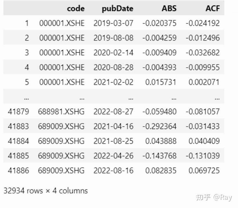
factor = basic[[&#39;code&#39;, &#39;pubDate&#39;, &#39;ABS&#39;, &#39;ACF&#39;]].dropna()
8.质量(Quality)(二)
未完待续…… |
|


 发表于 2023-1-14 12:45:10